Visualizing 2D and 3D superformulae equations with Julia and the Plots and Makie visualization packages.
Introduction 🔗
Superformula is a generic geometric transformation equation that can be used to describe a wide range of forms found in nature. It was first proposed by Johan Gielis as a generalization of the superellipse or Lamé curve and published in 2003 as an invited special paper in the American Journal of Botany.
I first came across it on Ed Nisley’s blog when I was looking for some interesting things to do with my recently restored HP 7475A pen plotter.
In polar coordinates, with $r$ and $φ$ the angle, Superformula can be expressed as:
$$ r\left(\varphi\right) = \left( \left| \frac{\cos\left(\frac{m\varphi}{4}\right)}{a} \right| ^{n_2} + \left| \frac{\sin\left(\frac{m\varphi}{4}\right)}{b} \right| ^{n_3} \right) ^{-\frac{1}{n_{1}}} $$
A further generalization of Superformula, SuperformulaU was proposed one year later in 2004 by Uwe Stöhr to allow the creation of rotationally asymmetric and nested structures. In SuperformulaU, the parameter $m$ is replaced by two independent factors, $y$ and $z$:
$$ {r\left(\varphi \right)=\left(\left|{\frac {\cos \left({\frac {y\varphi }{4}}\right)}{a}}\right|^{n_{2}}+\left|{\frac {\sin \left({\frac {z\varphi }{4}}\right)}{b}}\right|^{n_{3}}\right)^{-{\frac {1}{n_{1}}}}} $$
In this post, I use Superformula as what I think is a visually pretty pleasing example to explore the basics of Julia’s plotting capabilities.
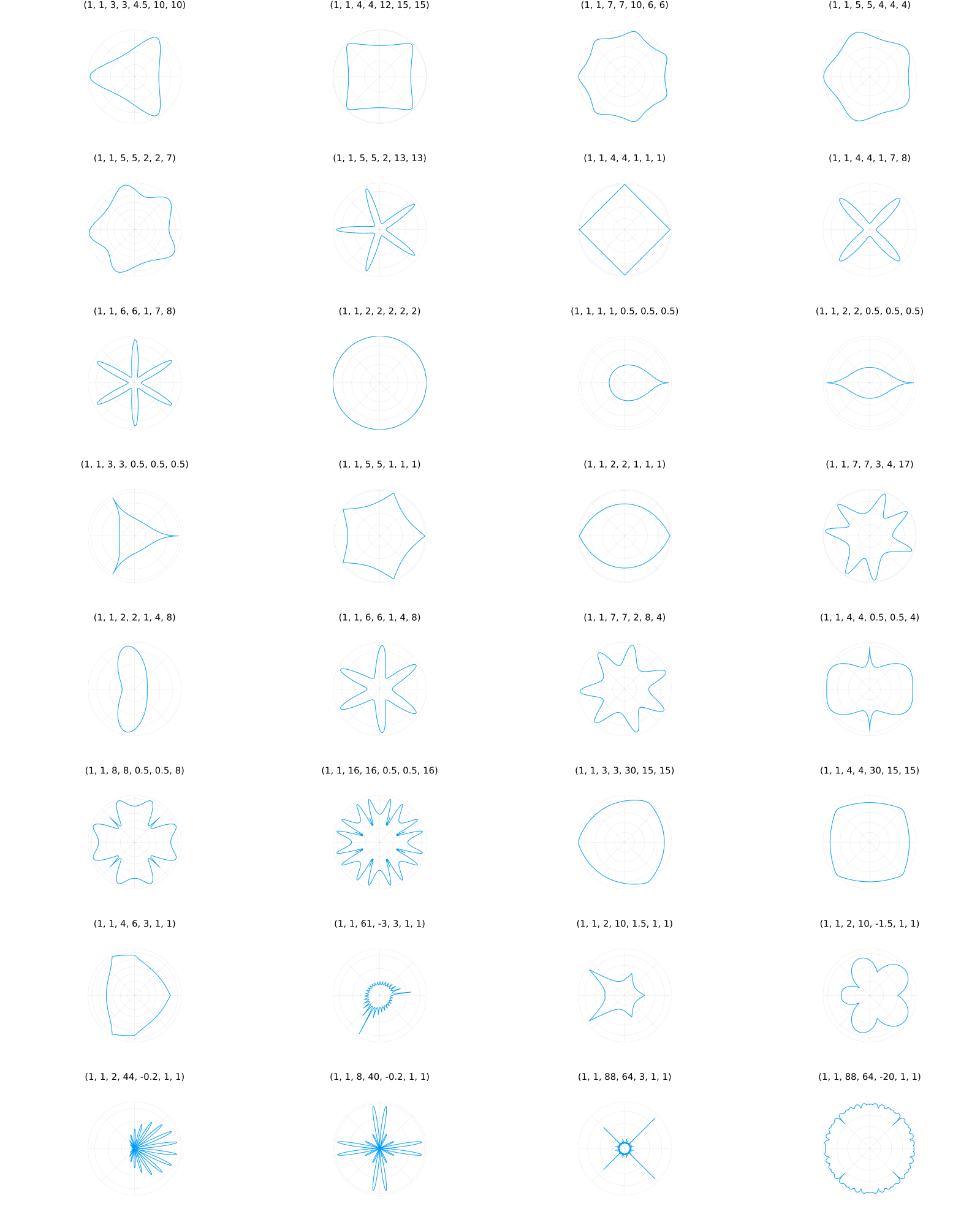
Superformula 2D 🔗
The Julia code below implements the generalized SuperformulaU in two dimensions. It uses the Plots package and subplot layout to generate a couple of interesting shapes for different values of $x$, $y$, $n_1$, $n_2$ and $n_3$.
🪲 There is a bug in Plots (tested with v1.30.2) that completely breaks subplot layouts for polar projection plots if the
PlotlyJSbackend is selected. You’ll have to use the defaultgr()backend for this to work.
The resulting plot looks like this (click to enlarge):
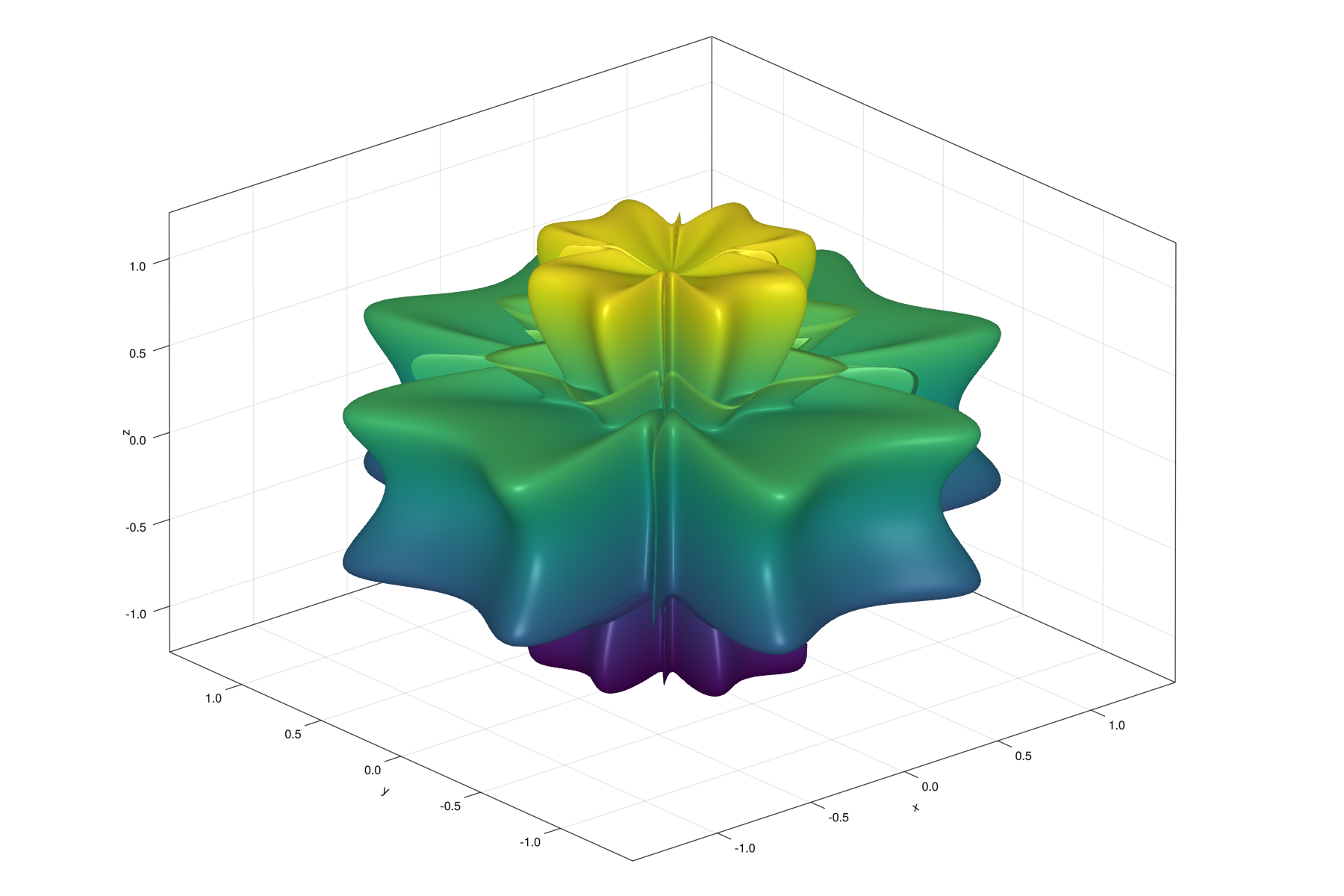
Superformula 3D 🔗
To calculate a 3D parametric surface, we can simply calculate the spherical product of two superformulae $r_{1}$ and $r_{2}$. The $x$, $y$, and $z$ coordinates of a surface point are defined by the following relations:
$$x=r_{1}(\theta)\cos \theta \cdot r_{2}(\phi )\cos \phi$$ $$y=r_{1}(\theta)\sin \theta \cdot r_{2}(\phi )\cos \phi$$ $$z=r_{2}(\phi )\sin \phi$$
where the spherical latitude $\phi$ varies between $−π/2$ and $π/2$ and the longitude $\theta$ between $−π$ and $π$.
The resulting plot looks like this (click to enlarge):